Optimization of Beam Profile in Fluid-Structure Interaction

The test case combines fluid-structure interaction with optimization in a simple but effective way. The cost function is well defined, has a definite global minimum, and its evaluation requires the solution of a strongly coupled fluid-structure interaction problem. The individual problems are easily solved while the coupled problem sets requirements to the efficient coupling of the different subproblems. One of the biggest challenges of the case is to find a surface presentation that allows sufficient freedom in design and also enables the use of efficient optimization techniques. The test case may be used to provide a reference solution for the verification of software components for multi-physical optimization problems. Even though the case itself is not real, it may help in the development and testing of tools needed for industrial fluid-structure interaction problems.
Objectives:
The aim is to optimize the geometry of an elastic beam so that it bends as little as possible under the pressure and traction forces resulting from viscous incompressible flow. The profile of the beam has an effect both on the flow and the structural stiffness of the beam, respectively. The case includes three different variations. The first case is fully linear and involves only one-directional coupling between the models. The linearity is achieved by neglecting the inertial forces in the Navier-Stokes equation, and by setting the beam to be so stiff that its bending is so small that its influence on the flow does not need to be taken into account. This also means that there is no geometric nonlinearities in the problem. The second variation increases the Reynolds number but the coupling is still one-directional. The third variation includes geometric nonlinearities in the elasticity equation, and nonlinearity resulting from the fluid-structure coupling. The optimum profile of the linear problem will not depend on any of the material parameters while in the nonlinear case the optimum profile will be parameter dependent.
Requirements: Incompressible Navier-Stokes solver for laminar flow
Elasticity solver for large displacement
Method to extent elastic deformarmation of the to the geometry of the fluid mesh
Capability to solve fluid-structure-interaction problems
Computational domain: Rectangular domain of size 102
Standing beam (height = 1, total area = 0.3), the tip of the beam located at x=25
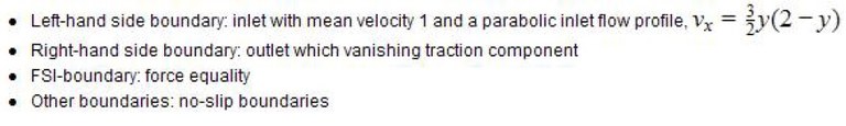
Boundary and/or initial conditions for computations:
Boundary conditions:
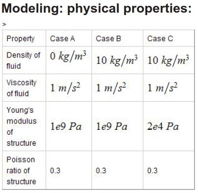
Material Parameters:
Solid
Fluid
Optimization:
The goal is to optimize the shape of the left-hand side wall of the beam so that its height and area stay fixed. The width at the bottom may freely vary as long as the other constraints are met.
Design parameters:
The standing beam: height = 1, total area = 0.3. The left and right walls may be assumed to be smooth.
Objective function definition:
f=max(|u|)
Results:
The different solutions may be compared to each other using 0D, 1D and 2D data.. Below the different data for comparison is defined.
Scalar values:
- Maximum displacement on the beam at optimum
- Maximum displacement on the beam at rectangular shape
- Displacement reduction factor
- Area of the optimized beam
- Parametrization of the left wall pro file
Ideally the results are saved in a format which enables that the results are studied with the same software. For line plotting the natural format is a table where the columns represent different fields and the rows different nodes.
- The shape of the left side wall as a [y;x] table
- The displacement on the left side wall as [y;ux] table
- The pressure on the left side wall as [y;p] table
Contour plots:
Ideally the results are saved in a format which enables that the results are compared within the same visualization software. For 2D the contour plots this format could be the VTK format (or its newer XML generalizations) that enable visualization with all VTK derived software such as Paraview.
- Contour plot of absolute velocity
- Contour plot of pressure
- Contour plot of displacement
Additional information:
The results may also discuss the different numerical methods and optimization algorithms used. For successful comparison this information is however, not required.
-
Defined by Peter Råback, 2006.